Project-2
ST 558 Project 2
Project maintained by kafrazi2 Hosted on GitHub Pages — Theme by mattgraham
ST 558 Project 2
Kaylee Frazier and Rebecca Voelker 10/31/2021
- Introduction
- Exploratory Data Analysis (EDA)
- Create New Variables for EDA
- Graphical summary of shares by Content Length and Weekday vs. Weekend
- Graphical and Numerical summary of shares by Weekday vs. Weekend
- Graphical and Numerical summary of shares by Title Polarity and Length
- Numerical summary of shares by day_of_the_week
- Bar chart of shares by day of the week
- Summary table of shares by number of images
- Scatter plot of the image number and shares.
- Scatter plot of the number of videos and shares.
- Modeling
- Model Comparison and Selection
Introduction
The following is an analysis of online news popularity across a variety of channels. This analysis covers the following 6 data channels:
- Lifestyle
- Entertainment
- Business
- Social Media
- Tech
- World
The following report analyzes the # of shares of a particular piece of content as a function of a variety of variables, including;
- Number of Images in the Content (num_imgs)
- Number of Videos in the Content (num_videos)
- Week vs. Weekend Publications (is_weekend)
- Number of Words in the Content (n_tokens_content)
- Number of Words in the Title (n_tokens_titel)
- Polarity of the Content Title (abs_title_sentiment_polarity)
A few new variables were created, as well, which are described alongside the respective R Code.
As a part of our analysis, we modeled each of our predictive variables linearly, as well as via Random Forest and Boosted Tree Models. The various models were then compared against one another to select our final model, which was fit to our test data.
#Read in Libraries

library(tidyverse)
library(readr)
library(ggplot2)
library(randomForest)
library(shiny)
library(dplyr)
library(caret)
## Check Working Directory Path
getwd()
## [1] "C:/Users/Rebecca/OneDrive/Desktop/ST 558/Repos/Project2"
## Read in Raw Data Using Relative Path
rawData <- read_csv(file = "./project2_rawdata.csv")
rawData
## # A tibble: 39,644 x 61
##    url        timedelta n_tokens_title n_tokens_content n_unique_tokens
##    <chr>          <dbl>          <dbl>            <dbl>           <dbl>
##  1 http://ma~       731             12              219           0.664
##  2 http://ma~       731              9              255           0.605
##  3 http://ma~       731              9              211           0.575
##  4 http://ma~       731              9              531           0.504
##  5 http://ma~       731             13             1072           0.416
##  6 http://ma~       731             10              370           0.560
##  7 http://ma~       731              8              960           0.418
##  8 http://ma~       731             12              989           0.434
##  9 http://ma~       731             11               97           0.670
## 10 http://ma~       731             10              231           0.636
## # ... with 39,634 more rows, and 56 more variables:
## #   n_non_stop_words <dbl>, n_non_stop_unique_tokens <dbl>,
## #   num_hrefs <dbl>, num_self_hrefs <dbl>, num_imgs <dbl>,
## #   num_videos <dbl>, average_token_length <dbl>, num_keywords <dbl>,
## #   data_channel_is_lifestyle <dbl>,
## #   data_channel_is_entertainment <dbl>, data_channel_is_bus <dbl>,
## #   data_channel_is_socmed <dbl>, data_channel_is_tech <dbl>, ...
## Create a New Variable to Data Channel
rawDataNew <- rawData %>% mutate(data_channel =   if_else(data_channel_is_bus == 1, "Business",
       if_else(data_channel_is_entertainment == 1, "Entertainment",
               if_else(data_channel_is_lifestyle == 1, "Lifestyle",
                      if_else(data_channel_is_socmed == 1, "Social Media",
                              if_else(data_channel_is_tech == 1, "Tech", "World"))))))

## Subset Data for Respective Data Channel
subsetData <- rawDataNew %>% filter(data_channel == params$data_channel)

## Create Training and Test Data Sets
set.seed(500)
trainIndex <- createDataPartition(subsetData$shares, p = 0.7, list = FALSE)

trainData <- subsetData[trainIndex,]
testData <- subsetData[-trainIndex,]

trainData
## # A tibble: 5,145 x 62
##    url        timedelta n_tokens_title n_tokens_content n_unique_tokens
##    <chr>          <dbl>          <dbl>            <dbl>           <dbl>
##  1 http://ma~       731             13             1072           0.416
##  2 http://ma~       731             10              370           0.560
##  3 http://ma~       731              8             1207           0.411
##  4 http://ma~       731             13             1248           0.391
##  5 http://ma~       731              8              266           0.573
##  6 http://ma~       731             12             1225           0.385
##  7 http://ma~       731             10              633           0.476
##  8 http://ma~       731             10             1244           0.418
##  9 http://ma~       731             14             1237           0.424
## 10 http://ma~       731             10             1081           0.428
## # ... with 5,135 more rows, and 57 more variables:
## #   n_non_stop_words <dbl>, n_non_stop_unique_tokens <dbl>,
## #   num_hrefs <dbl>, num_self_hrefs <dbl>, num_imgs <dbl>,
## #   num_videos <dbl>, average_token_length <dbl>, num_keywords <dbl>,
## #   data_channel_is_lifestyle <dbl>,
## #   data_channel_is_entertainment <dbl>, data_channel_is_bus <dbl>,
## #   data_channel_is_socmed <dbl>, data_channel_is_tech <dbl>, ...
testData
## # A tibble: 2,201 x 62
##    url        timedelta n_tokens_title n_tokens_content n_unique_tokens
##    <chr>          <dbl>          <dbl>            <dbl>           <dbl>
##  1 http://ma~       731             12              989           0.434
##  2 http://ma~       731             11               97           0.670
##  3 http://ma~       731             11             1154           0.427
##  4 http://ma~       731              8              331           0.563
##  5 http://ma~       731             14              290           0.612
##  6 http://ma~       731             10             1036           0.430
##  7 http://ma~       731              6              174           0.692
##  8 http://ma~       731             11              214           0.645
##  9 http://ma~       731              9              944           0.433
## 10 http://ma~       731              9             1070           0.422
## # ... with 2,191 more rows, and 57 more variables:
## #   n_non_stop_words <dbl>, n_non_stop_unique_tokens <dbl>,
## #   num_hrefs <dbl>, num_self_hrefs <dbl>, num_imgs <dbl>,
## #   num_videos <dbl>, average_token_length <dbl>, num_keywords <dbl>,
## #   data_channel_is_lifestyle <dbl>,
## #   data_channel_is_entertainment <dbl>, data_channel_is_bus <dbl>,
## #   data_channel_is_socmed <dbl>, data_channel_is_tech <dbl>, ...
=======
Exploratory Data Analysis (EDA)
Create New Variables for EDA
#Create New Variable that Measures Title Length
trainData <- trainData %>% mutate(TitleLength = if_else(n_tokens_title <= 10, "Short Title",
  if_else(n_tokens_title <= 15, "Medium Title", "Long Title")))

#Create New variable using weekday_is_() variables
trainDataNew <- trainData %>% mutate(day_of_the_week =   if_else(weekday_is_monday == 1, "Monday",
       if_else(weekday_is_tuesday == 1, "Tuesday",
               if_else(weekday_is_wednesday == 1, "Wednesday",
                      if_else(weekday_is_thursday == 1, "Thursday",
                              if_else(weekday_is_friday == 1, "Friday",
                                      if_else(weekday_is_saturday == 1, "Saturday", "Sunday"
                                              )))))))
trainDataNew
## # A tibble: 5,145 x 64
##    url        timedelta n_tokens_title n_tokens_content n_unique_tokens
##    <chr>          <dbl>          <dbl>            <dbl>           <dbl>
##  1 http://ma~       731             13             1072           0.416
##  2 http://ma~       731             10              370           0.560
##  3 http://ma~       731              8             1207           0.411
##  4 http://ma~       731             13             1248           0.391
##  5 http://ma~       731              8              266           0.573
##  6 http://ma~       731             12             1225           0.385
##  7 http://ma~       731             10              633           0.476
##  8 http://ma~       731             10             1244           0.418
##  9 http://ma~       731             14             1237           0.424
## 10 http://ma~       731             10             1081           0.428
## # ... with 5,135 more rows, and 59 more variables:
## #   n_non_stop_words <dbl>, n_non_stop_unique_tokens <dbl>,
## #   num_hrefs <dbl>, num_self_hrefs <dbl>, num_imgs <dbl>,
## #   num_videos <dbl>, average_token_length <dbl>, num_keywords <dbl>,
## #   data_channel_is_lifestyle <dbl>,
## #   data_channel_is_entertainment <dbl>, data_channel_is_bus <dbl>,
## #   data_channel_is_socmed <dbl>, data_channel_is_tech <dbl>, ...
Graphical summary of shares by Content Length and Weekday vs. Weekend
#Convert is_weekend to a Factor
trainData$is_weekend <- factor(trainData$is_weekend)

#Table of Publications on Weekdays vs. Weekend
table(trainData$is_weekend)
##
##    0    1
## 4491  654
#Create a Scatter Plot of # of Words by Shares
g1 <- ggplot(trainData, aes(x = n_tokens_content, y = shares)) +
  geom_point(aes(col = is_weekend)) +
    geom_smooth(method = "lm", aes(col = is_weekend))
g1
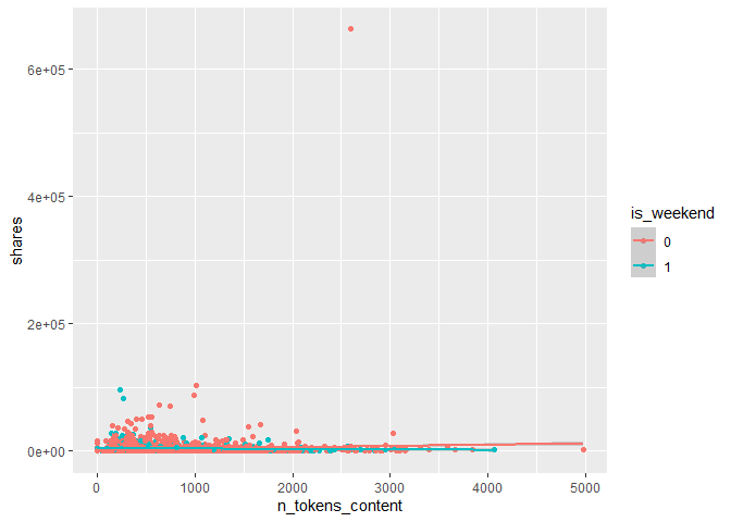
We can inspect the trend of shares as a function of the number of words (tokens) in the content. If the points show an upward trend, then content with more words tends to be shared more often.If we see a negative trend then content with more words tends to be shared less often. The color-coding specifies if the content was published on a Weekday or Weekend.
Graphical and Numerical summary of shares by Weekday vs. Weekend
#Create a Box Plot of Weekend vs. Weekday by Shares
g2 <- ggplot(trainData, aes(x = is_weekend, y = shares)) +
  geom_boxplot()
g2
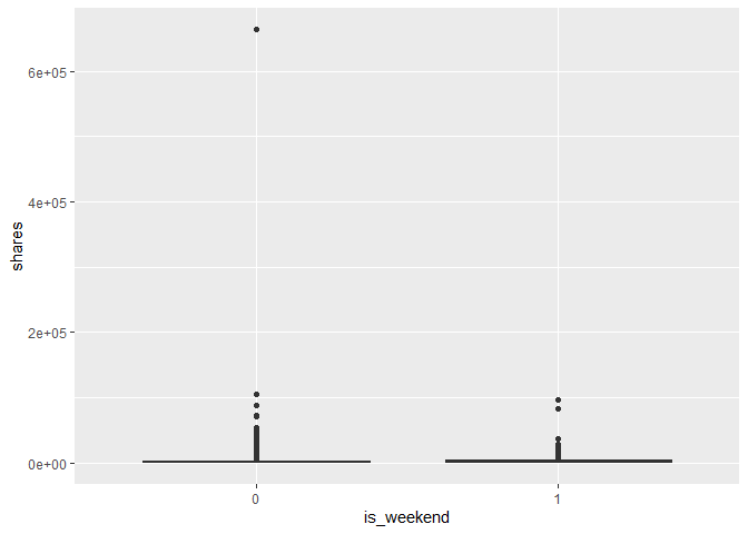
#Generate a Numerical Summary of Data Summarized in our Box Plot
trainData %>% group_by(is_weekend) %>% summarise(min = min(shares), med = median(shares), max = max(shares), mean = mean(shares))
## # A tibble: 2 x 5
##   is_weekend   min   med    max  mean
##   <fct>      <dbl> <dbl>  <dbl> <dbl>
## 1 0             36  1600 663600 3025.
## 2 1            119  2200  96100 3798.
We can inspect the trend of shares as a function of Weekday vs. Weekend Publications. The statistics show the Minimum, Maximum, Median, and Average # of Shares by Week (Published During the Week) vs. Weekend (Published During the Weekend)
Graphical and Numerical summary of shares by Title Polarity and Length
table(trainData$n_tokens_title)
##
##   4   5   6   7   8   9  10  11  12  13  14  15  16  17  18  19  20
##   3  27 130 335 596 860 940 881 662 397 201  71  20  15   5   1   1
# Create a Scatter Plot of Polarity of Title by Shares
g3 <- ggplot(trainData, aes(x = abs_title_sentiment_polarity, y = shares)) +
  geom_point(aes(col = TitleLength)) +
    geom_smooth(method = "lm", aes(col = TitleLength))
g3
## `geom_smooth()` using formula 'y ~ x'
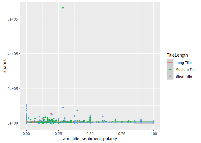
# Numerical Correlation of Polarity of Title by Shares
cor(trainData$abs_title_sentiment_polarity, trainData$shares)
## [1] 0.01795861
We can inspect the trend of shares as a function of the polarity of the title of the content. If the points show an upward trend, then content with a more polarizing title (positive or negative) tends to be shared more often.If we see a negative trend then content with more a more polarizing title (positive or negative) tends to be shared less often. The color-coding specifies the length of the title. The correlation, shows us the numerical value of the correlation between our predictor variable(s) and response
Numerical summary of shares by day_of_the_week
#find mean, median, and standard deviation of shares by day_of_the_week
daySummary <-trainDataNew %>% group_by(day_of_the_week) %>% summarise(avg_shares = mean(shares), med_shares = median(shares), sd_shares = sd(shares))

#print out numerical summary
daySummary
## # A tibble: 7 x 4
##   day_of_the_week avg_shares med_shares sd_shares
##   <chr>                <dbl>      <dbl>     <dbl>
## 1 Friday               3005.       1800     5660.
## 2 Monday               2865.       1650     3958.
## 3 Saturday             3703.       2200     6068.
## 4 Sunday               3924.       2200     6386.
## 5 Thursday             2704.       1600     3716.
## 6 Tuesday              2891.       1600     4767.
## 7 Wednesday            3610.       1600    21517.
In the summary plot you can see which days had the highest and lowest average shares, median shares, and look at the standard deviation to see which day had the largest range of shares.
Bar chart of shares by day of the week
#create a basic plot with x and y variables
g5 <- ggplot(data = trainDataNew, aes(day_of_the_week, shares))
#make the plot a bar chart
g5 + geom_col(aes(fill = day_of_the_week), position = "dodge") +
#change the angle of the words to fit
  guides(x = guide_axis(angle = 45)) +
  labs(title = "Day of the Week vs. Shares") +
#get rid of legend
  theme(legend.position = "none")
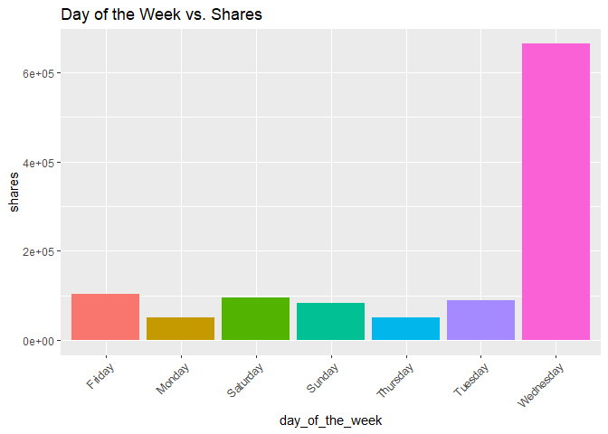
In this bar chart of day of the week vs. shares, you can see which days had the greatest total number of shares and which had the lowest.
Summary table of shares by number of images
#create summary table with different ranges of images
imagesSummary <- trainData %>% group_by(cut(num_imgs, c(min(num_imgs), 10, 20, 40, 60, 80, max(num_imgs)))) %>% summarise(avg_shares = mean(shares), med_shares = median(shares), sd_shares = sd(shares))

#rename column name
names(imagesSummary)[names(imagesSummary) == "cut(num_imgs, c(min(num_imgs), 10, 20, 40, 60, 80, max(num_imgs)))"] <- "image_number"

#print out numerical summary
imagesSummary
## # A tibble: 6 x 4
##   image_number avg_shares med_shares sd_shares
##   <fct>             <dbl>      <dbl>     <dbl>
## 1 (0,10]            3050.       1700    12021.
## 2 (10,20]           3624.       1900     7096.
## 3 (20,40]           2526.       1600     3047.
## 4 (40,60]           3639.       1600     5157.
## 5 (60,65]           2250        2250      778.
## 6 <NA>              3207.       1700     5229.
In the summary plot you can see if the amount of images affected the average, median, and standard deviation of shares.
Scatter plot of the image number and shares.
#create basic plot with x and y
g6 <- ggplot(trainData, aes(x = num_imgs, y = shares))
#make it a scatter plot with regression line
g6 + geom_point() +
    geom_smooth(method = "lm")
## `geom_smooth()` using formula 'y ~ x'
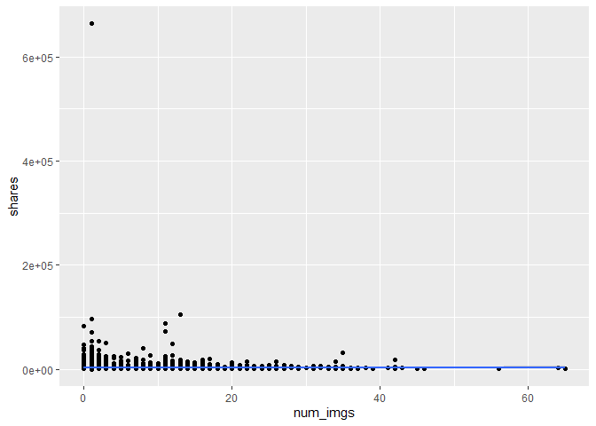
In this scatter plot of the number of images vs. shares, you can see the relationship between the two variables. If it shows an upward trend, articles with more images tend to be shared more often. If the trend is negative, then articles with less images tend to be shared more.
Scatter plot of the number of videos and shares.
#create basic plot with x and y
g7 <- ggplot(trainData, aes(x = num_videos, y = shares))
#make it a scatter plot with regression line
g7 + geom_point() +
    geom_smooth(method = "lm")
## `geom_smooth()` using formula 'y ~ x'
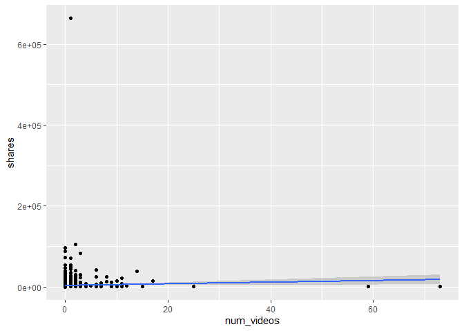
In this scatter plot of the number of videos vs. shares, you can see the relationship between the two variables. If it shows an upward trend, articles with more videos tend to be shared more often. If the trend is negative, then articles with less videos tend to be shared more.
Modeling
Linear Regression Models
A linear regression model allows for easy prediction of a response variable. It’s goal is to figure out which variables are significant predictors of the response variable and how do they impact it.
This Multiple Linear Regression Model looks at the # of Shares as a function of the # of Words in the Content AND whether or not the Content was published on a Weekend (0 = No, 1 = Yes)
## Convert is_weekend to Numeric
trainData$is_weekend <- as.numeric(trainData$is_weekend)

## Fit Multiple Linear Regression Model
fitLM1 <- train(shares ~ n_tokens_content + is_weekend, data = trainData, method = "lm", trControl = trainControl(method = "cv", number = 10))
fitLM1
## Linear Regression
##
## 5145 samples
##    2 predictor
##
## No pre-processing
## Resampling: Cross-Validated (10 fold)
## Summary of sample sizes: 4630, 4632, 4630, 4631, 4632, 4629, ...
## Resampling results:
##
##   RMSE      Rsquared     MAE
##   7317.619  0.004021453  2442.413
##
## Tuning parameter 'intercept' was held constant at a value of TRUE
This Multiple Linear Regression Model looks at the # of Shares as a function of the # the Quadratic of Title Polarity Sentiment AND the Title Length (Short, Medium, Long)
## Fit Multiple Linear Regression Model
fitLM2 <- train(shares ~ abs_title_sentiment_polarity^2 + TitleLength, data = trainData, method = "lm", trControl = trainControl(method = "cv", number = 10))
fitLM2
## Linear Regression
##
## 5145 samples
##    2 predictor
##
## No pre-processing
## Resampling: Cross-Validated (10 fold)
## Summary of sample sizes: 4630, 4632, 4629, 4632, 4630, 4630, ...
## Resampling results:
##
##   RMSE      Rsquared     MAE
##   7229.547  0.002447625  2435.09
##
## Tuning parameter 'intercept' was held constant at a value of TRUE
This multiple linear regression model looks at day of the week, number of images, and number of videos as predictors and shares as response.
#create fit using shares as response, day_of_the_week, num_imgs, and num_videos as the predictors
fitLM3 <- train(shares ~ day_of_the_week + num_imgs + num_videos, data = trainDataNew,
#method is linear model
              method = "lm",
#center and scale the data
                preProcess = c("center", "scale"),
#10 fold cross validation
              trControl = trainControl(method = "cv", number = 10))
fitLM3
## Linear Regression
##
## 5145 samples
##    3 predictor
##
## Pre-processing: centered (8), scaled (8)
## Resampling: Cross-Validated (10 fold)
## Summary of sample sizes: 4631, 4631, 4631, 4631, 4630, 4631, ...
## Resampling results:
##
##   RMSE      Rsquared     MAE
##   7131.692  0.006515172  2435.885
##
## Tuning parameter 'intercept' was held constant at a value of TRUE
Random Forest Model
Random forest modeling is a type of ensemble model that creates multiple trees from bootstrap samples without using all the predictors and a random subset of predictors for each sample. It then averages the results from the multiple trees.
#use train function
rfFit <- train(shares ~ day_of_the_week + num_imgs + num_videos + n_tokens_content, data = trainDataNew,
#use rf method
               method = "rf",
#5 fold validation
               trControl = trainControl(method = "cv", number = 5),
#consider values of mtry
               tuneGrid = data.frame(mtry = 1:4))
rfFit
## Random Forest
##
## 5145 samples
##    4 predictor
##
## No pre-processing
## Resampling: Cross-Validated (5 fold)
## Summary of sample sizes: 4115, 4116, 4116, 4116, 4117
## Resampling results across tuning parameters:
##
##   mtry  RMSE      Rsquared     MAE
##   1     8228.654  0.005026855  2451.642
##   2     8851.499  0.005181669  2492.305
##   3     9263.370  0.005272177  2526.752
##   4     9745.361  0.004626937  2588.931
##
## RMSE was used to select the optimal model using the smallest value.
## The final value used for the model was mtry = 1.
Boosted Tree Model
Boosted modeling is a type of ensemble model that grows subsequent trees off of modified version of the original data. Any resulting predictions are updated as your Boosted Tree Model grows, based on criteria like the # of Subsequent Trees, Shrinkage Paramter, etc.
n.trees <- c(5, 10, 25, 100)
interaction.depth <- 1:4
shrinkage <- 0.1
n.minobsinnode <- 10

df <- expand.grid(n.trees = n.trees, interaction.depth = interaction.depth, shrinkage = shrinkage, n.minobsinnode = n.minobsinnode)

boostFit <- train(shares ~ abs_title_sentiment_polarity^2 + TitleLength, data = trainData, method = "gbm", trControl = trainControl(method = "cv", number = 5), tuneGrid = df)

boostFit$results
boostFit$bestTune
Model Comparison and Selection
#Add New Variables (Title Length and Day of the Week) to Test Data
testData <- testData %>% mutate(TitleLength = if_else(n_tokens_title <= 10, "Short Title",
  if_else(n_tokens_title <= 15, "Medium Title", "Long Title")))

testData <- testData %>% mutate(day_of_the_week =   if_else(weekday_is_monday == 1, "Monday",
       if_else(weekday_is_tuesday == 1, "Tuesday",
               if_else(weekday_is_wednesday == 1, "Wednesday",
                      if_else(weekday_is_thursday == 1, "Thursday",
                              if_else(weekday_is_friday == 1, "Friday",
                                      if_else(weekday_is_saturday == 1, "Saturday", "Sunday"
                                              )))))))

## Obtain RMSE on Test Data for Linear Models
predLM1 <- predict(fitLM1, newdata = testData)
postResample(predLM1, obs = testData$shares)
##         RMSE     Rsquared          MAE
## 4.268902e+03 1.332561e-02 1.982352e+03
predLM2 <- predict(fitLM2, newdata = testData)
postResample(predLM2, obs = testData$shares)
##         RMSE     Rsquared          MAE
## 4.250155e+03 4.568622e-03 2.273942e+03
predLM3 <- predict(fitLM3, newdata = testData)
postResample(predLM3, obs = testData$shares)
##         RMSE     Rsquared          MAE
## 4.258650e+03 2.991412e-03 2.253009e+03
## Obtain RMSE on Test Data for Random Forest Model
predRF <- predict(rfFit, newdata = testData)
postResample(predRF, testData$shares)
##         RMSE     Rsquared          MAE
## 4.306242e+03 2.587582e-03 2.277307e+03
## Obtain RMSE on Test Data for Boosted Fit Model
predBoost <- predict(boostFit, newdata = testData)
postResample(predBoost, testData$shares)
##         RMSE     Rsquared          MAE
## 4.279073e+03 7.523759e-04 2.259464e+03